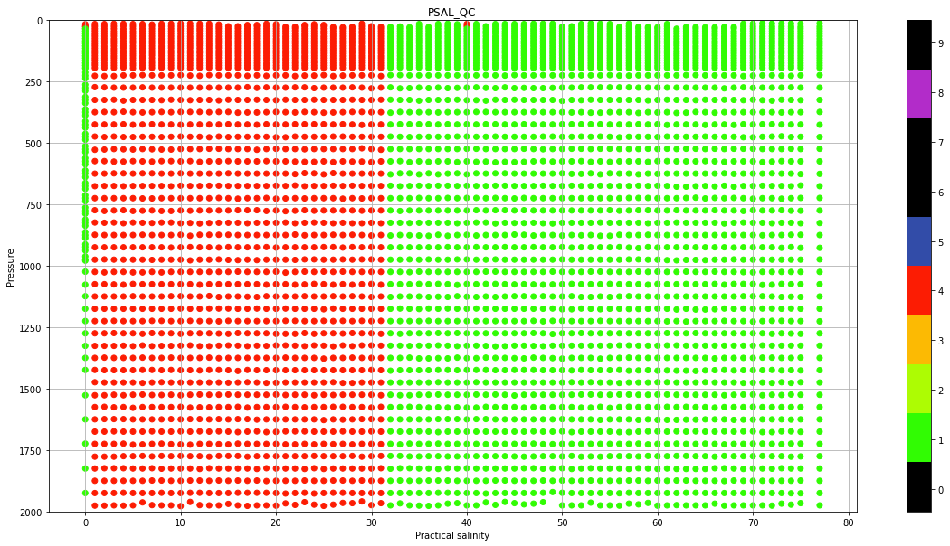
Real Time quality control data

Real Time quality control data#

Real-Time quality control is a set of automatic procedures that are performed at the National Data Acquisition Centers (DACs) to carry out the first quality control of the data. There are a total of 19 tests that aim, to say, easy to identify anomalies in the data. The subtle anomalies, that need a lot of expertise and time to discern between sensor malfunctioning and natural variability, are left for the Delayed-Mode quality control.

The results of the Real-Time tests are summarized in what is called the quality control flags. Quality control flags are an essential part of Argo.

Quality Control flags#

Each observation after the RT quality control has a QC flag associated, a number from 0 to 9, with the following meaning:

QCflag	Meaning	Real time description
0	No QC performed	No QC performed
1	Good data	All real time QC tests passed
2	Probably good data	Probably good
3	Bad data that are potentially correctable	Test 15 or Test 16 or Test 17 failed and all other real-time QC tests passed. These data are not to be used without scientific correction. A flag ‘3’ may be assigned by an operator during additional visual QC for bad
4	Bad data	Data have failed one or more of the real-time QC tests, excluding Test 16. A flag ‘4’ may be assigned by an operator during additional visual QC for bad data that are not correctable.
5	Value changed	Value changed
6	Not currently used	Not currently used
7	Not currently used	Not currently used
8	Estimated	Estimated value (interpolated, extrapolated or other estimation)
9	Missing value	Missing value

First, let’s see how this information is stored in the NetCDF files

import numpy as np
import netCDF4
import xarray as xr

import matplotlib as mpl
import matplotlib.cm as cm
from matplotlib import pyplot as plt
%matplotlib inline

Before accesing the data, let’s create some usefull colormaps and colorbar makers to help us to understand the QC flags

qcmap = mpl.colors.ListedColormap(['#000000', 
                                   '#31FC03', 
                                   '#ADFC03', 
                                   '#FCBA03', 
                                   '#FC1C03',
                                   '#324CA8', 
                                   '#000000', 
                                   '#000000', 
                                   '#B22CC9', 
                                   '#000000'])
def colorbar_qc(cmap, **kwargs):
    """Adjust colorbar ticks with discrete colors for QC flags"""
    ncolors = 10
    mappable = cm.ScalarMappable(cmap=cmap)
    mappable.set_array([])
    mappable.set_clim(-0.5, ncolors+0.5)
    colorbar = plt.colorbar(mappable, **kwargs)
    colorbar.set_ticks(np.linspace(0, ncolors, ncolors))
    colorbar.set_ticklabels(range(ncolors))
    return colorbar

## QC flags for data accessed by date open the daily data set from the 11th november 2019

dayADS = xr.open_dataset('../../Data/atlantic_ocean/2020/11/20201111_prof.nc')

Besides the core variables, TEMP, PSAL and PRES, we also have the variables TEMP_ADJUSTED, PSAL_ADJUSTED and PRES_ADJUSTED, which correspond to DM, or calibrated data. However, here we keep the focus on the Real-Time data, and in the next section, we will use the calibrated data.

Let’s begin by plotting the location of all the data.

Location#

fig, ax = plt.subplots(figsize=(20,10))
sc = ax.scatter(dayADS.LONGITUDE, dayADS.LATITUDE, cmap=qcmap)
ax.grid()

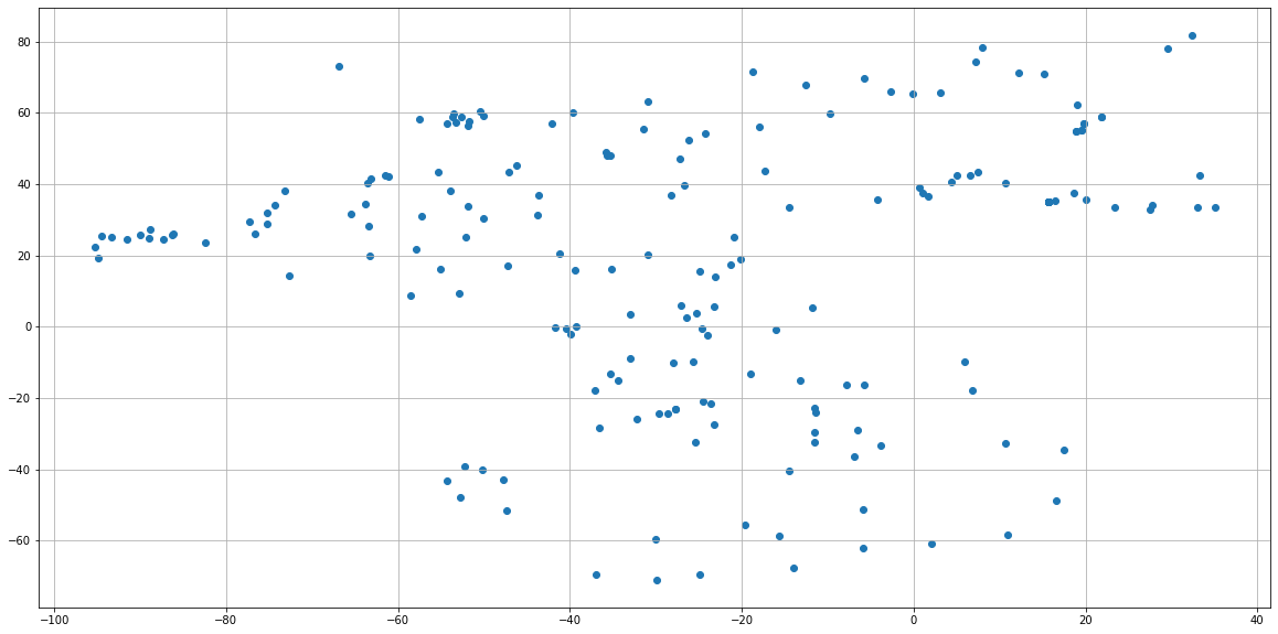
../../_images/227d20c850abea1a0544fa911c540c28a9c271bbb96244328f321f3f5796231c.png

If we want to get a better map, we need cartopy, although we could skip this step.

import cartopy.crs as ccrs
import cartopy

fig,ax = plt.subplots(figsize=(20,10),subplot_kw={'projection': ccrs.PlateCarree()})
ax.plot(dayADS.LONGITUDE,dayADS.LATITUDE,'ob')

ax.add_feature(cartopy.feature.LAND)
ax.add_feature(cartopy.feature.COASTLINE, edgecolor='white')
ax.set_title(f"Data from {dayADS.JULD[0].values.astype('datetime64[D]')}")

ax.gridlines(draw_labels=True, dms=True, x_inline=False, y_inline=False)
ax.set_xlim([-100, 40]);    

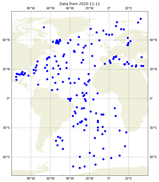
../../_images/a9085272becf5511e3addf9921c438163c4493735dbb62872e5375ebd038da11.png

and now the actual data, a TS diagram

fig, ax = plt.subplots(figsize=(20,10))
sc = ax.scatter(dayADS.PSAL, dayADS.TEMP, cmap=qcmap)
ax.grid()

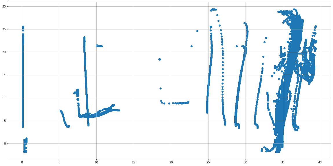
../../_images/2df03aac21e20ab3e1e1afd52de907f3766e8b13d1bfd9bb17ab70b902e20228.png

some data is obviously wrong, hence, let’s check if all the QC is Good data

pres=dayADS.PRES
lon=dayADS.LONGITUDE+pres*0

fig, ax = plt.subplots(figsize=(20,10))
sc = ax.scatter(lon, pres, c=dayADS.PSAL_QC, vmin=0, vmax=9, cmap=qcmap)
colorbar_qc(qcmap, ax=ax)
ax.grid()
ax.set_ylim(0,2000)
ax.invert_yaxis()
ax.set_xlabel(f"{dayADS.PSAL.long_name}")
ax.set_ylabel('Pressure')
ax.set_title('PSAL_QC');

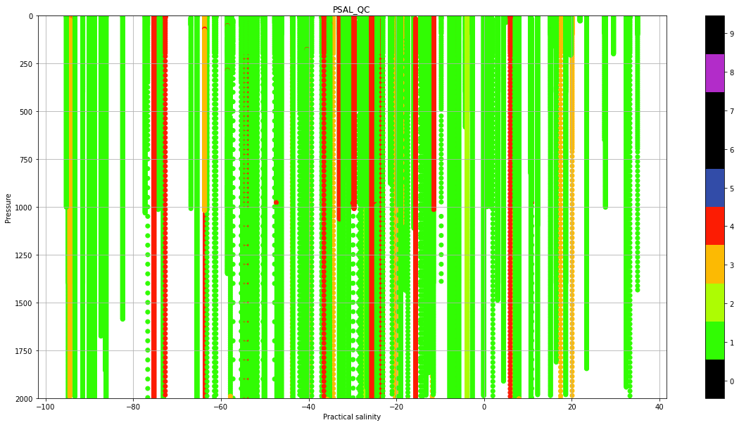
../../_images/be17db628c13694c09c39c41c685413aded708102329fa8386eb53323b669d09.png

There a lot of profiles with Quality Flag (QC) that indicate bada data. Now, we will plot the same TS diagram, but color coding the data bvased on the Quality flags.

fig, ax = plt.subplots(figsize=(20,10))
sc = ax.scatter(dayADS.PSAL.where(dayADS.PSAL_QC.values.astype(float) == 0), 
                dayADS.TEMP.where(dayADS.PSAL_QC.values.astype(float) == 0), 
                c=dayADS.PSAL_QC.where(dayADS.PSAL_QC.values.astype(float) == 0), vmin=0, vmax=9, cmap=qcmap)

sc = ax.scatter(dayADS.PSAL.where(dayADS.PSAL_QC.values.astype(float) == 1), 
                dayADS.TEMP.where(dayADS.PSAL_QC.values.astype(float) == 1), 
                c=dayADS.PSAL_QC.where(dayADS.PSAL_QC.values.astype(float) == 1), vmin=0, vmax=9, cmap=qcmap)

sc = ax.scatter(dayADS.PSAL.where(dayADS.PSAL_QC.values.astype(float) == 2), 
                dayADS.TEMP.where(dayADS.PSAL_QC.values.astype(float) == 2), 
                c=dayADS.PSAL_QC.where(dayADS.PSAL_QC.values.astype(float) == 2), vmin=0, vmax=9, cmap=qcmap)


sc = ax.scatter(dayADS.PSAL.where(dayADS.PSAL_QC.values.astype(float) == 3), 
                dayADS.TEMP.where(dayADS.PSAL_QC.values.astype(float) == 3), 
                c=dayADS.PSAL_QC.where(dayADS.PSAL_QC.values.astype(float) == 3), vmin=0, vmax=9, cmap=qcmap)


sc = ax.scatter(dayADS.PSAL.where(dayADS.PSAL_QC.values.astype(float) == 4), 
                dayADS.TEMP.where(dayADS.PSAL_QC.values.astype(float) == 4), 
                c=dayADS.PSAL_QC.where(dayADS.PSAL_QC.values.astype(float) == 4), vmin=0, vmax=9, cmap=qcmap)

colorbar_qc(qcmap, ax=ax)
ax.grid()

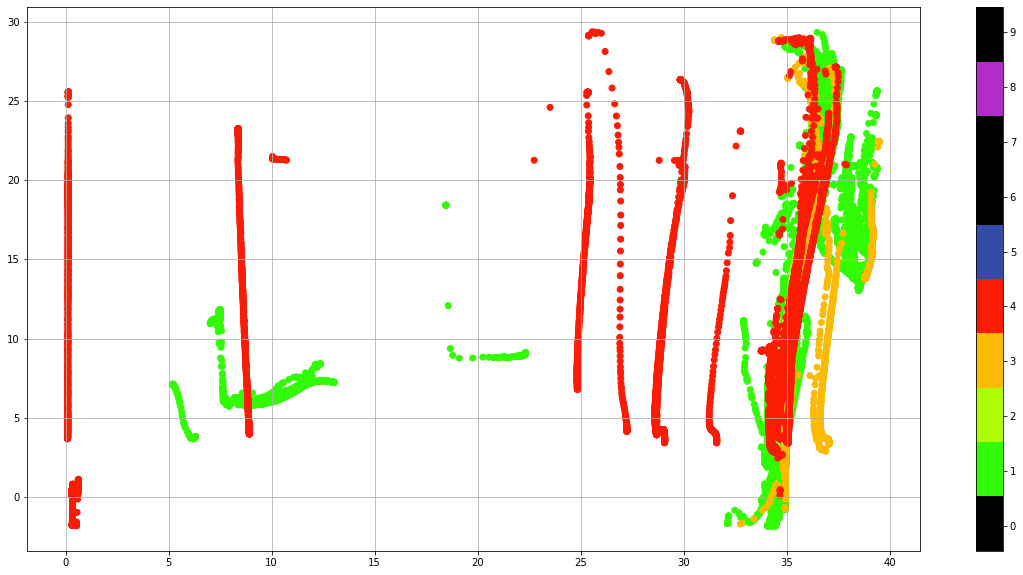
../../_images/1981b8d06b12a70bf24aceb0d65da03fecde610871247af63d4c22ec1d8a0c19.png

Using the QC flags we could just select the good data (QC=1) or, if we are familiar with the data, we can keep all the data that could be good, (QC=0, 1, 2 or 5) and decide what to do with the suspicius data.

Addtionally there is a Global quality flag for each one of the parameters, that indicate the percentage of good data in the profile. For salinitiy this global quality flag is PROFILE_PSAL_QC and it

Flag	Description
A	N = 100% , all profile levels contain good data
B	75% <= N < 100%
C	75% <= N < 100%
D	75% <= N < 100%
E	75% <= N < 100%
F	N = 0%, no profile levels have good data

A N = 100%; All profile levels contain good data. B 75% <= N < 100% C 50% <= N < 75% D 25% <= N < 50% E 0% < N < 25%

Example : PROFILE_TEMP_QC = A : the temperature profile contains only good values = C : the salinity profile contains 50% to 75% good values

dayADS.LONGITUDE.where(dayADS.PROFILE_PSAL_QC.values.astype(str) == 'A')

fig,ax = plt.subplots(figsize=(20,10),subplot_kw={'projection': ccrs.PlateCarree()})
ax.plot(dayADS.LONGITUDE.where(dayADS.PROFILE_PSAL_QC.values.astype(str) == 'A'), 
        dayADS.LATITUDE.where(dayADS.PROFILE_PSAL_QC.values.astype(str) == 'A'),
        'ob')

ax.plot(dayADS.LONGITUDE.where(dayADS.PROFILE_PSAL_QC.values.astype(str) == 'B'), 
        dayADS.LATITUDE.where(dayADS.PROFILE_PSAL_QC.values.astype(str) == 'B'),
        'or')

ax.plot(dayADS.LONGITUDE.where(dayADS.PROFILE_PSAL_QC.values.astype(str) == 'C'), 
        dayADS.LATITUDE.where(dayADS.PROFILE_PSAL_QC.values.astype(str) == 'D'),
        'or')
ax.plot(dayADS.LONGITUDE.where(dayADS.PROFILE_PSAL_QC.values.astype(str) == 'E'), 
        dayADS.LATITUDE.where(dayADS.PROFILE_PSAL_QC.values.astype(str) == 'E'),
        'or')
ax.plot(dayADS.LONGITUDE.where(dayADS.PROFILE_PSAL_QC.values.astype(str) == 'F'), 
        dayADS.LATITUDE.where(dayADS.PROFILE_PSAL_QC.values.astype(str) == 'F'),
        'or')

#ax.set_title(f"Data from {Rtraj.PLATFORM_NUMBER.values.astype(str)}")
ax.add_feature(cartopy.feature.LAND)
ax.add_feature(cartopy.feature.COASTLINE, edgecolor='white')

ax.gridlines(draw_labels=True, dms=True, x_inline=False, y_inline=False)
ax.set_xlim([-100, 40]);  

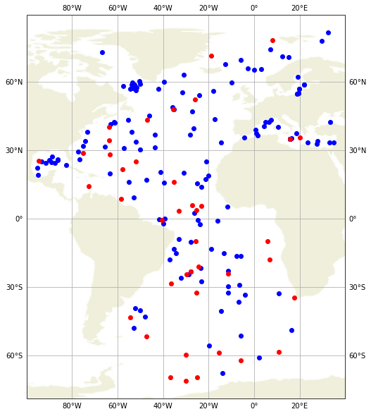
../../_images/a5f74d1e0d8465713a6c38626f7d1f8f251d9cf3db44b8fda96d03e415ea67e7.png

## QC flags for data accessed by float

iwmo = 1900379
#iwmo = 6900230
file = f"/Users/pvb/Dropbox/Oceanografia/Data/Argo/Floats/{iwmo}/{iwmo}_prof.nc"
dayADS = xr.open_dataset(file)

fig, ax = plt.subplots(figsize=(20,10))
sc = ax.scatter(dayADS.PSAL, dayADS.TEMP, cmap=qcmap)
ax.grid()

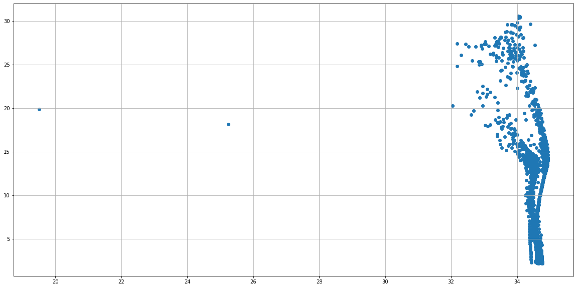
../../_images/d15a6072806f36696b41a7e5386c0295c9f593200c7fd94f0b98e6b171bc680f.png

pres=dayADS.PRES
cycle=dayADS.CYCLE_NUMBER+pres*0

fig, ax = plt.subplots(figsize=(20,10))
sc = ax.scatter(cycle, pres, c=dayADS.PSAL_QC, vmin=0, vmax=9, cmap=qcmap)
colorbar_qc(qcmap, ax=ax)
ax.grid()
ax.set_ylim(0,2000)
ax.invert_yaxis()
ax.set_xlabel(f"{dayADS.PSAL.long_name}")
ax.set_ylabel('Pressure')
ax.set_title('PSAL_QC');  

../../_images/90d02f4cd318cf7b8c90a5775eff85e0f147964618c4c34c19a3d407c301810e.png

Real Time quality control data

Contents

Real Time quality control data#

Quality Control flags#

Location#